An Image, according to Wikipedia, is an artifact of something. From what I know, I define an image as a visual representation of an object or event. Immortality objectified.
According to the handout given by Dr. Soriano, there are four basic image types. These are the Binary images, which are basically black OR white images, Grayscale images, which are black AND white images, Truecolor images, which are images that have RGB colors, and the Index images, which are also colored images, but these colors are represented by numbers which denote the index of the colors in a colormap. In the wake of advancing technology, imaging techniques are also advancing, and thus image types have become advanced as well. Here are some of the more advanced image types;
- HDR, or High Dynamic Range, type of images - These images are simply grayscale images but they require more than 8-bit memory to be truly appreciated.
- Multi or Hyperspectral images - These are images that have more bands than the common 3 (RGB).
- 3D images - As the name suggests, these are images that have 3 dimensions. A common example is the MRI images.
- Temporal Images or Videos - These are basically what we see in cinemas, moving pictures
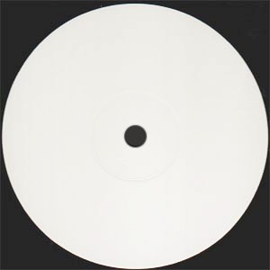
Figure 1: Binary Image type. This is as close as I can get in finding a visually looking Binary image type, an image of black OR white colors. Image taken here.
 Figure 2: Grayscale Image Type. This is what you would visually expect from a grayscale image type, an image of black AND white colors. Image taken here.
 Figure 3: Truecolor image type. A beautiful image of RGB colors.
 Figure 4: Index image types. There are numbers that represent a corresponding color, indicated by the colormap.
Now that we have identified some of the image types, let me proceed to the different image formats. The most common image format out there is the '.jpeg'. JPEG stands for 'Joint Photographic Expert Group', the ones who developed and promoted the use of this file format. '.bmp', '.png', '.tif' are some of the more common file formats created by man. Of course there are other file formats, but they are less popular because interestingly, according to Dr. Soriano, people have to pay in order to use them, and nowadays people just don't want to pay. There are variations in file formats because obviously, each has its ups and downs.Wikipedia, whether you like it or not, has it all covered,so, go and check it out.
As cameras gain more and more pixel, storage and transmission of the images they produce CAN become a problem. For that, two image file formats can be used, depending on the application of the image, to store and transmit images.
- Lossy Image Compression - some of the images' information are lost. This loss of information though may not be such a bad thing because depending on the setting and what the observer is looking for, that person may not even notice the loss of information. Its greatest upside is, because of the loss of information, the resulting image is very compact making it easier to store and transmit. '.jpg' and '.gif' are examples of lossy image formats.
- Lossless Image Compression - all of the images' information are preserved. This type of format is essential for application wherein even a small dot on the image can mean something, as is the case of medical imaging. '.tif' and '.png' are examples of lossless image compression
For this activity, we were made to 'play' around with some of the images we can find from our laptop and from the net.
Figure 5: Original graph from activity 1. Untouched image.
Figure 5 was taken from our first activity. In any case, let us investigate this image.By using the size() function found in scilab, its size matrix can be obtained, which is (389 rows x 860 columns x 3). Looking closer at figure 5, it kind of looks like a grayscale image, but it actually is a truecolor image type. Notice that in the size matrix, there is the number 3, it actually indicates the presence of RGB (Red, Green, Blue) colors, which means, that figure 5 really is a truecolor image.
The following figures are some of the images taken from the web and its corresponding information. The information was derived using the imfinfo() function also found in scilab.
 Filesize : 46829
Format: JPEG
Width: 343
Height: 504
Depth: 8
StorageType: Truecolor
Resolution unit: Centimeter
Xresolution: 100
Yresolution: 100
Figure 6: Batman and his information. Image taken here.

Filesize: 76162
Format: GIF
Width: 382
Height:381
Depth: 8
StorageType: indexed
Numberofcolors: 256
Resolution Unit: centimeter
Xresolution: 72
Yresolution: 72
Figure 7: A basketball and its information. Image taken here
 Filesize: 263222
Format: BMP
Width: 512
Height: 512
Depth: 8
StorageType: indexed
Numberofcolors: 256
Resolution unit: centimeter
Xresolution: 0
Yresolution: 0
Figure 8: The beautiful Lena and her information. Image taken here.
What happens if we convert a truecolor image type into a binary or grayscale image type? By using im2bw() and im2gray() functions found in scilab, figure 9 has the answer.


Figure 9: This is a truecolor image (leftmost) of me converted into a grayscale image (middle) and into a binary image (rightmost). The binary image type has level of 0.5
Figure 9 shows a transition from truecolor image to a grayscale image, and also to a binary image. The binary image type has a level of 0.5 meaning that any pixel value of the truecolor image less than 50 percent of the maximum pixel value would be converted to zero (black) and any pixel value of the truecolor image more than 50 percent of the maximum pixel value would be converted to 1 (white).
Lets go back to figure 5, the original graph from activity 1. Figure 10 shows the grayscale image type version of figure 5.

Figure 10: Grayscale image type version of figure 5
As you can probably observe, Figure 10 and Figure 5 kind of looks exactly the same, but don't be mistaken, figure 5 actually is a truecolor image type, even though it lacks the prominent RGB colors of a truecolor image. On the other hand, figure 10 is an image composed of Black and White colors only, so, even though they look exactly alike, they are very much different.
By getting the histoplot of the pixel values of figure 10, we could actually determine the frequency of pixel values used for this grayscale version. And ultimately, by using the im2bw() function, specifically, its 'level' argument, we can 'clean' this image to the point that it will look a lot better than its original image.
 Figure 11. A 'clean' version of the original graph in figure 5. By using a level of 0.45, I was able to erase some of the unnecessary background smudges from the original graph.
This activity ranks as one of the most enjoyable activities I have done, mainly because I get to manipulate something very common today, and that is an image. So, all in all, for technical correctness, I believe I only deserve a score of 4 because I posted this blog entry late, and for Quality of presentation, I believe I got a score of 5 because of the clarity of both the images and the captions. So, 9 out of 10? Not bad, at least for me. On to the next activity.
 Figure 2: Grayscale Image Type. This is what you would visually expect from a grayscale image type, an image of black AND white colors. Image taken here.
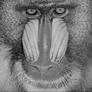
 Figure 3: Truecolor image type. A beautiful image of RGB colors.
 Figure 4: Index image types. There are numbers that represent a corresponding color, indicated by the colormap.
 Filesize : 46829

 Filesize: 263222


 Figure 11. A 'clean' version of the original graph in figure 5. By using a level of 0.45, I was able to erase some of the unnecessary background smudges from the original graph.
No comments:
Post a Comment