Color Image Processing

If there is one thing a lay man needs to know about digital cameras, its that per pixel in the camera, the color captured by a certain digital color camera is the integral of the product of the spectral power distribution of the incident light source , the surface reflectance and the spectral sensitivity of the camera

and where

, i = [Red, Green and Blue]. K is the balancing constant equal to the inverse of the camera output when a white object is shown.

Digital Cameras nowadays have the White Balance feature wherein the user can adjust the white balancing constants appropriate for certain conditions. White balancing simply implies that when a camera captures an image, white will (and should) appear white in the captured image. The following are some of the settings a user can set the White Balance to

• Sun - for sunny and bright outdoors
• Cloud - for a cloudy day
• Light Bulb - for incandescent lighting
• Fluorescent lamp - for fluorescent lighting

If setting the proper White Balance becomes quite tedious, the 'AWB' setting, which stands for Automatic White Balancing, can instead be used. Other symbols such as the '6500K' can also be seen, this stands for the color temperature of the light. Again, the reason as to why setting the white balance to its proper condition is recommended to make white appear white with the rest of the colors properly rendered.

There are two well known algorithms that can perform automatic white balancing, the White Patch Algorithm and the Gray World Algorithm. The key idea in Automatic White Balancing is to determine the output of the camera for a white object. In white patch algorithm, an image is taken under a wrongly white balanced setting, then use the RGB values of a known white object as the divider (divide this to the obtained R,G,B of the image). On the other hand, Gray world algorithm, assumes that the average color of the world is gray, hence take the average of the R,G and B of the wrongly white balanced image and use this average r,g and b value as the divider (divide this to the obtained R,G and B of the image).

The following figures are the result of implementing the Automatic White Balancing algorithms on several wrongly white balanced images.

Figure 1: 'Auto' White Balance Setting (left image). The image in the middle is the result of implementing the White Patch Algorithm. The image on the right is the result of implementing the Gray World Algorithm.

Figure 2: 'Daylight' White Balance Setting (left image). The image in the middle is the result of implementing the White Patch Algorithm. The image on the right is the result of implementing the Gray World Algorithm.


Figure 3: 'Fluorescent' White Balance Setting (left image). The image in the middle is the result of implementing the White Patch Algorithm. The image on the right is the result of implementing the Gray World Algorithm.


Figure 4: 'Tungsten' White Balance Setting (left image). The image in the middle is the result of implementing the White Patch Algorithm. The image on the right is the result of implementing the Gray World Algorithm.

Before I proceed, I would like to thank May Ann Tenorio for the images in figures 1 to 4 (unprocessed images).

It can be observed that whether the White Patch algorithm or the Gray World Algorithm, is used white did indeed appear white. Using the gray world algorithm though supersaturates the image (the image became very bright) relative to the image produced when the white patch algorithm is used. For this case, it is better to implement the white patch algorithm instead of the gray world algorithm.

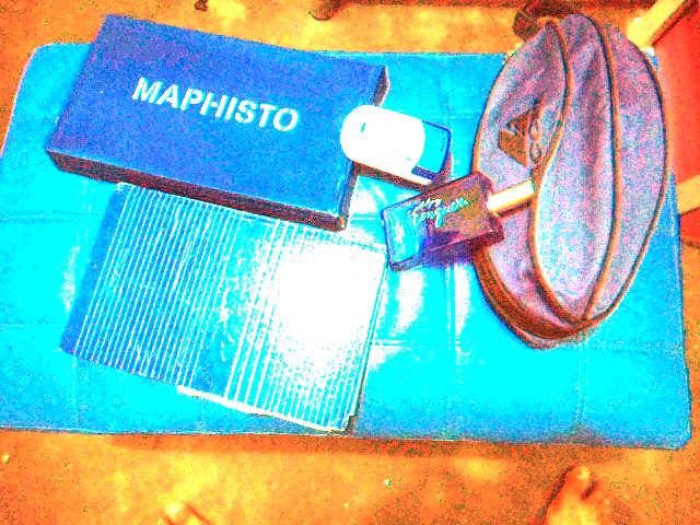
Figure 5: Objects of the same hue (color) under 'Fluorescent' white balance setting. Left image is the unprocessed image captured under 'Fluorescent' white balance setting. Middle image is the result after applying the white patch algorithm. Rightmost image is the result after applying the gray world algorithm.

Before I proceed, I would like to thank Aivin Solatorio for the image (unprocessed).

Figure 5 shows an image of objects of the same hue (color) captured under 'Fluorescent' white balance setting. It can be observed that using the white patch algorithm is so much better in 'white balancing' the image compared to using the gray world algorithm wherein parts of the images are again supersaturated. So all in all, it is recommended to use the White Patch Algorithm rather than the Gray world algorithm in the Auto White Balance feature of any camera.

Again, I would like to thank May Ann Tenorio and Aivin Solatorio for the images. I would also like to acknowledge my discussions with Tino Borja, Arvin Mabilangan, Gino Leynes and Dr. Soriano.

--
Technical Correctness: 5/5
Quality of Presentation: 5/5

Image Compression

As the title implies, this post/activity is all about compressing an image. This activity makes use of the concept of Principal Component Analysis (PCA). Images can be compressed using bases of sinusoids of different frequencies along the x and y axis. So basically, an image can be represented and then compressed by the superposition of weight basis images (PCA eigenfunctions, or in this case, eigenimages).

First of all, open an image in scilab as a grayscale image. For this post, consider the image in figure 1.

Figure 1: Grayscale image to be compressed. The image size is 480x640

The next step is to cut this image into 10x10 block images. Therefore 3072 10x10 block images are formed from figure 1. Then, concatenate each block by using img(:), given that img is a 10x10 block. The resulting matrix is a 3072x100 matrix, where 3072 indicates the number of 10x10 blocks and 100 indicates the number of pixels in that block.

Next is to apply PCA on the 3072x100 matrix, defined as the matrix x. PCA can be implemented in scilab by using the function pca(x). Upon implementation of the PCA, three matrices will be given ([lamda, facpr, comprinc]).

The first matrix, lamda, is a px2 matrix, where p is the number of variables/pixels (in this case, p = 100). The first column of this matrix gives the eigenvalues and the second column gives the ratio of that corresponding eigenvalue.

The second matrix, facpr, shows the principal factors or the eigenvectors.

The third matrix, comprinc, gives the principal components, or basically the coefficient corresponding to a certain eigenvector.

The idea is, depending on how many nonzero eigenvectors will be used to reconstruct the image, an eigenvector (from 1 column in fracpr) will be multiplied to its corresponding coefficient for all blocks (in this case 3072 blocks). For example, if only the top three eigenvectors (meaning these eigenvectors are the top three contributors) are used, then per block, only the three corresponding coefficients are used. Let an eigenvector be noted as V and its corresponding coefficient, c, again if only three V's are used then per block, (V1*c1 + V2*c2 + V3*c3) is computed to reconstruct that block. The resulting matrix, in this case, is a 3072x100 matrix, where, again, 3072 is the number of blocks and 100 is the result of (V1*c1 + V2*c2 + V3*c3). From this matrix, all the information needed to reconstruct the image have been gathered. The final step is to return each row (there are 3072 rows) into 10x10 blocks once again, and thus the image is reconstructed.

Compression occurs because, as stated earlier, only three eigenvectors are used, where as to fully reconstruct the image (meaning without loss), all 100 eigenvectors must be used.

The corresponding images are reconstructions of figure 1 by using different numbers of top eigenvectors.

Figure 2: Reconstruction by using only the top three eigenvectors. 297984 pixels are lost from 307200 pixels originally or 97% pecent loss.


Figure 3: Reconstruction by using only the top ten eigenvectors. 276480 pixels are lost from 307200 pixels originally or 90% pecent loss.


Figure 4: Reconstruction by using only the top 25 eigenvectors. 230400 pixels are lost from 307200 pixels originally or 75% pecent loss.


Figure 5: Reconstruction by using only the top 50 eigenvectors. 153600 pixels are lost from 307200 pixels originally or 50% pecent loss.


Figure 6: Reconstruction by using only the top 90 eigenvectors. 30720 pixels are lost from 307200 pixels originally or 10% pecent loss.


Figure 7: Reconstruction by using all the eigenvectors. 0 pixels are lost from 307200 pixels originally or 0% pecent loss.

The number of pixels lost can be computed by solving for the difference between the original number of pixels (in this case, 307200) and (the number of 10x10 blocks multiplied by the number of eigenvectors used). It can be observed that increasing the number of eigenvectors used decreases the number of pixels lost, but, it can also be observed from the images that at a certain number of eigenvector, the reconstructed image is already as identical as the original image (meaning, even with a number of pixels lost, the reconstructed image can still represent the original image) and this is the basis of compressing an image. Certain information or pixels are lost without greatly affecting the quality of the image.

Below is the source code used for this activity

//open the image and convert to grayscale
image = imread('C:\Documents and Settings\andy polinar\Desktop\ap 186\activities\activity 14\shadespic.jpg');
I = (image(:,:,1)+image(:,:,2)+image(:,:,3))/3;

simage = size(image);

//vectorizing the image, producing x
k = 0;
for r = 1:(simage(1)/10)
for c = 1:(simage(2)/10)
itemp = I(((10*r-9):(10*r)),((10*c-9):(10*c)));
xtemp = itemp(:);
k = c + (r-1)*(simage(2)/10);
x(k,:) = xtemp';
end
end

//implementing pca
[lambda,facpr,comprinc] = pca(x);

vectors = 90; //indicates the number of top eigenvectors to be used
scomprinc = size(comprinc);
sfacpr = size(facpr);
redim = zeros(((simage(1)*simage(2))/100),100);
for rcomprinc = 1:scomprinc(1);
temp = zeros(100,1);
for cfacpr = 1:vectors
mrc = facpr(:,cfacpr)*(comprinc(rcomprinc,cfacpr));
temp = temp+mrc;
end
temp = temp';
redim(rcomprinc,(1:100))=temp;
end

//reconstruction of the image
y = zeros(simage(1),simage(2));
k=0;
for r = 1:(simage(1)/10)
for c = 1:(simage(2)/10)
k = c + (r-1)*(simage(2)/10);
xtemp=redim(k,:);
y(((10*r-9):(10*r)),((10*c-9):(10*c))) = matrix(xtemp,10,10);
end
end

//computing for the number of pixels lost
originalmem = simage(1)*simage(2);
newmem = ((simage(1)*simage(2))/100)*vectors;
lost = originalmem - newmem;
lostpercent = ((originalmem - newmem)/originalmem)*100;

I would like to acknowledge my discussions with Arvin Mabilangan and Dr. Maricor Soriano.

--
Technical Correctness: 5/5
Quality of Presentation: 5/5

Color Image Segmentation

For this activity, the skill to pick out the region of interest (ROI) from the rest of the image is developed. Selection rules are based on the unique features of the ROI. One quick way to segment the ROI from the rest of the image is to convert the image into grayscale then set some threshold value to isolate the ROI, but this method does not always guarantee success. The case for grayscale images is that, more often than not, the ROI has the same or overlapping grayscale values as the background, making it relatively impossible to isolate the ROI for further processing.

Another way to segment images is by use of color, and its application can be seen in face and hand recognition, isolation of land cover in remote sensing, and cell identification in microscopy.

Inherently, 3D colored objects will have shading variations and in some extent this shadow variations can be thought of as differing brightness of the same color. It is recommended that the color space be represented not by RGB alone but by a coordinate system in which the brightness information is separated from the chromaticity (pure color) information. One such color space that can do this is the Normalized Chromaticity Coordinates or the NCC.

Consider an image, per pixel of that image, let its intensity be I = R+B+G (the primary colors). Then the NCC are

with r+g+b = 1. This implies that r,g, and b can only have values from 0 to 1, and the calculation of b is dependent of r and g, meaning b = 1 - r - g. With this, it is actually enough to represent chromaticity just by 2 coordinates (r and g). All in all, the color space has been transformed from the R G B to the r g I, where r and g contains the chromatic information and the I contains the brightness information.

Figure 1: Normalized Chromaticity Space. x-axis is red (r) and y-axis is green (g).

Figure 1 shows the NCC. Due to the transformation, the color information has been reduced from 3 dimensions to just 2. It can be observed that when r = 0 and g = 0, b = 1, indicating that the origin corresponds to blue. As observed in figure 1, any color can be represented in the NCC.

Parametric vs. Non-Parametric Probability Distribution

Segmentation based on color can be performed by determining the probability that a pixel, with a certain color belongs to a certain color distribution of interest. The color distribution of interest can be obtained by cropping a part of the image that contains the color distribution of interest.

Parametric

To indicate if a pixel belongs to the region on interest or not, its probability of being part of the ROI must be determined. Since the space/coordinates used contains r and g, a joint probability function (p(r)*p(g)) can be defined to test the likelihood of a pixel to belong to the ROI. For this experiment, it is assumed that the probability function is a Guassian distribution function given by

with p(g) being the same function but with a sigma (variance) and mean for g. , and , can be derived from the pixel samples of the cropped ROI using the stdev() and mean() functions respectively. r is the corresponding red color value of a certain pixel in the original image, and g in p(g) being the corresponding green color value of the same pixel. Depending on the value of p(r)*p(g), certain pixels will light up while others will be blackened. Figure 2 shows the result of applying this algorithm on an image of a rubix cube with the ROI being the yellow color enclosed in a rectangle.

Figure 2: Rubix Cube (left) taken from here. Right image is the result after applying the parametric algorithm.

Notice that in figure 2, although there is more than 3 yellow colored region, not all of them are highlighted, this is probably due to the different shading of the color yellow in the image.

Non-Parametric

Non-Parametric method makes use of the 2d color distribution histogram of an image and the specified ROI. The histogram itself is used to identify pixels (based on their color) that belongs to the ROI. Histogram backprojection can be used to give a certain pixel location (in the original image) its corresponding value based on the histogram of the cropped ROI. The code below is a sample code of implementing a 2d histogram in scilab. (souce code given by Dr. Soriano in her handout for this activity)

I = double(I); //I is the image of the region of interest
R = I(:,:,1); G = I(:,:,2); B = I(:,:,3);
Int= R + G + B;
Int(find(Int==0))=100000;
r = R./ Int; g = G./Int;
BINS = 32;
rint = round( r*(BINS-1) + 1);
gint = round (g*(BINS-1) + 1);
colors = gint(:) + (rint(:)-1)*BINS;
hist = zeros(BINS,BINS);
for row = 1:BINS
for col = 1:(BINS-row+1)
hist(row,col) = length( find(colors==( ((col + (row-1)*BINS)))));

end;
end;
scf(2); imshow(hist,[]);

Figure 3: 2d histogram of the Rubrix cube (left) and 2d histogram of the cropped ROI. Note that the y-coordinates in scilab are inverted.

Figure 3 shows the histogram of the image of the rubrix cube and the cropped ROI. Note that the y coordinates are inverted. This histogram correlates to the colors indicated in figure 1. Notice that the colors of the image and the cropped ROI match the colors indicated in the chromaticity space.

Figure 4: Result after applying the non parametric algorithm. The ROI is the yellow color.

Again, not all yellow colored regions are highlighted.

As observed there is quite a difference in using the parametric and non parametric methods to isolate the Region of Interest. The parametric method basically makes use of the probability distribution while the non parametric method makes use of the 2D color histogram of the image. The use of analytic functions in the parametric method is only as efficient as the fit of the PDF function used. On the other hand, no calculations are needed in the non parametric method, only a look-up of the histogram information.

For me, it is better to use the non-parametric method in isolating/segmenting the ROI from the rest of the image.

I would like to acknowledge my discussions with Arvin Mabilangan.

--
Technical Correctness: 4/5 (late posting)
Quality of Presentation: 5/5

Playing Notes by Image Processing. What You See is What You Hear.

Amazingly, musical notes can also be played in scilab. Consider the musical score sheet in figure 1.

Figure 1: Rain Rain Go Away music score sheet.

After some processing, scilab would be abe to play these notes out.

This video file plays the musical score sheet in figure 1. Again, this is to emphasize that the notes can be played by using the concepts learned in Image Processing. The problem can be solved in a freestyle manner. For this post, I will be discussing everything, in detail, what I used to play these notes. The important thing is, the computer reads the score sheet and then plays the notes.

The main concept I will be using for this activity is the correlation concept. How two patterns are correlated? The higher the correlation, the more similar are the patterns in question.

Lucky for us the score sheet is relatively 'clean', so no further 'cleaning' is required.

First I cropped or copied the pattern of a half note and a quarter note (Figure 2 and 3 respectively). These cropped images will be used later to implement the correlation concept.

Figure 2: half note


Figure 3: quarter note

I open the score sheet, the half note and the quater note in scilab as grayscale images, using the gray_imread('filename/filepath') function. It is important to note that the half note and the quarter note must have the same size as the score sheet. Plus, the location of these notes must be at the center of the image, I can't emphasize it enough, the notes (half note and quarter note) must be at the center of their respective images.
The next step is to derive the corresponding FT's of the images. This is done by using the fft2(image) function.
The next step is to correlate the musical score sheet with the notes individually. This step helps in distinguishing the notes in the original musical score sheet in figure 1. Click here to review the concept of correlation.
Figure 4 shows the correlation between the scoresheet and the half note.

Figure 4: Correlation between the original score sheet and the half note.

Apparently, the difference between the half note and the quarter note is not that big because as figure 4 shows, even the quarter notes in the score sheet have high correlation with the half note. This can only mean that further processing is required.

Figure 5: Binarized image of the Correlation between the original score sheet and the half note.
This has a threshold value of 0.9

The next thing I did to further distinguish the half notes and the quarter notes in the original score sheet was to binarize the image as shown in figure 5. Then I observed that in figure 5, the half notes only have one pixel in size left, whereas the quarter notes have more than 1 pixel in size. With this in mind, I collected all the pixel location information of those 1 pixel size dots and labeled them as the half notes.

Figure 6 shows the correlation between the scoresheet and the quarter notes.

Figure 6: Correlation between the original scoresheet and the quarter note.

Much like the case in figure 4, figure 6 requires further processing to properly distinguish the notes. So, again, I binarized the image in figure 6, which is shown in figure 7.

Figure 7: Binarized image of the correlation between the original score sheet and the quarter notes.

As can be seen in figure 7, what remains are the points where the quarter notes are located. So, I collected all of their pixel locations and labeled them as quarter notes.

After collecting all of the necessary informations (the notes and their locations), I arranged them in such a way that their arrangement or order in the original score sheet are preserved. So basically, the column part of their pixel location indicates which notes should be played first. And the row part of their pixel location indicates in what frequency they should be played (A,B,C,D,E,F,G). The duration or how long they should be played is indicated by the correlation part.

Now that all of the necessary things are in hand (the notes, the order in which to play them, the frequency they should be played at, and the duration of how long they should be played), there is only one thing left to do, and that is to play music. In scilab, notes can be played by using the sound() function. A function that represents sound is also needed to play the notes and in simple terms, sound can be represented as a sine wave, hence a sin(frequency, time(=soundsec(time))) function is used, and depending on the frequency, different tones/pitch can be heard. The function soundsec() is used to indicate the duration of the note to be played. All in all, the note can be played by using this function: sound([function with the representation of sound]).

I would like to acknowledge my discussions with Arvin Mabilangan and Gino Leynes.

--
Technical Correctness: 4/5 (late posting)
Quality of Presentation: 5/5

Binary Operations

It is important in image-based measurements that the region of interest (ROI) must be well segmented from the background. This can be done by either edge detection (defining contours) or by specifying the ROI as blobs.

Now, binarizing an image simplifies the separation of the background from the ROI provided that the optimum threshold is implemented by first examining the image histogram. One commonly encountered problem in doing this process is the possibility of overlapping grayscale values of the ROI and the background, which entails further cleaning of the resulting image by use of morphological operations. With the use of the closing and opening operator, unwanted holes can be closed up and unnecessarily touching blobs can be separated.

Consider figure 1, imagine that these holes are cells and the objective is to find an estimate of the area of each cell.

Figure 1: An image of scattered punch paper digitized using a flat bed scanner. These holes could represent cells imaged under a microscope.

Now, image processing is very ideal for automating repetitive tasks and therefore, large images such as in figure 1 could be cut up into smaller sub images, and the procedure can then be implemented onto all subimages. Note that the subimages can overlap each other. This is very practical because in actual cancer screening, the task requires processing several samples from one subject.

Figure 2: Nine 256x256 pixel size subimages. Each subimage is subject to the prodecure used to determine the area of each hole.

The Procedure/Algorithm.

Consider the first subimage located at the 'topleft-most' of figure 2. Again, the objective is to find the best estimate for the area of each hole. The first priority is to separate the background from the ROI and this could be done by binarizing the image. By examining the histogram of this image, the background can be separated from the ROI. Figure 3 shows the histogram of the image.

Figure 3: Histogram of the subimage. Conveniently, this is also the histogram of the other subimages. The x-axis are the grayscale values while the y-axis are the frequencies.

By examining figure 3, the threshold value for the im2bw() function is set at 0.835. Conveniently, this histogram is basically the histogram of the other subimages and thus the threshold value 0.835 is used for all subimages.

Figure 4: Binarized Image.

Notice that binarizing the image to separate the background from the ROI is not that efficient. Unwanted holes can still be seen, and thus further 'cleaning' of the image is required. For this purpose, the closing and the opening operator can be used to close up unwanted holes and disconnect unnecessarily connected blobs. The closing operator simply dilates the image with a structuring element, then erode the resulting image with the same structuring element. On the other hand, the opening operator simply erodes the image first with a structuring element and then dilates the resulting image with the same structuring element. Again, Closing = Dilate then Erode, Opening = Erode then Dilate. To review the dilate and erode function, click here.

Since the ROIs are blobs in the shape of a circle, it is logical to use a structuring element also circlular in shape. Figure 5 shows the cleaned subimages using the opening and closing operator.

Figure 5: 'Cleaned' Binarized subimges. By using the Opening and Closing operator, holes were closed and connecting blobs were disconnected.

Admittedly, not all connected blobs are disconnected and not all blobs retained their circular shape but that's tolerable.

The next step is to estimate the area (in terms of pixel count) of each individual cell/blob. This can be done by using the bwlabel() function of scilab. What this function does is to label connecting blobs and number them accordingly. Then by counting the number of pixels included in a particular blob, the area of that particular blob is obtained (Note that the number of pixels is considered to be the area). Doing this for all the blobs in all the subimages, an estimate of the area can be derived. Figure 6 shows the histogram for all the computed area.

Figure 6: Histogram for the computed areas. x-axis are the areas (in pixel count) and the y-axis are the frequencies.

From Figure 6, it can deduced that the area is around 500 pixels. In order to get an accurate estimate, the outliers must be neglected, Figure 7 shows a 'cropped' histogram of the areas.

Figure 7: Cropped Histogram.

Solving for the mean() of this graph, the estimate for the area of each hole/cell/blob is computed.

The computed area (in pixel count) is 528.38 pixels with a standard deviation of 17.76 pixels. Of course the histogram in figure 6 can be cropped into different ranges but the important thing is to get the best estimate for the area. Cropping the histogram in figure 6 into a very small range would become trivial and noncredible, crop it into a very large range and the standard deviation becomes very large and thus the estimated area becomes inaccurate.

Application.

Cosinder the image in figure 8. Notice that some holes are bigger than the other. These bigger holes can be thought of as the cancer cells. The objective is to isolate these cancer cells.

Figure 8: An image of scattered punch papers but with holes larger than the others.

By implementing the same procedure as previously discussed, the bigger holes can be isolated. Again, the procedure goes like this, cut up the image into 256x256 pixels size, then binarize the image, then 'clean' up the binarized image, use bwlabel() to label and number each blob, then determine the area of each blob by counting the number of pixels included in a particular blob. Of course if the objective is just to isolate the cancer cells, represented by the bigger holes, then there is no need to use the bwlabel(). The important thing here is to create a structuring element with the same area as the area of the 'common' holes just derived. Then by implementing the opening operator on each blob, the common blobs, as well as the connected blobs can be removed. Figure 9 highlights the bigger holes which can be thought of as cancer cells.

Figure 9: Isolated cancer cells.

Again, admittedly, the isolated cancer cells are not perfectly circular in shape, and this could be accounted for by the somewhat 'imperfect' structuring element used, or by the binarizing technique implemented. It is acknowledged though that indeed the bigger holes were isolated and therefore if these were cancer cells, then the cancer cells have just been identified.

I would like to acknowledge my discussions with Dr. Soriano, BA Racoma, and Dennis Diaz.

--
Technical Correctness: 4/5 (late posting)
Quality of Presentations: 5/5