Image Enhancement by Histogram Manipulation

The histogram of a grayscale image is actually the gray level probability distribution function or the PDF of the grayscale image if the histogram is normalized by the total number of pixels. Why is this important? Because by manipulating the histogram, the quality of the image can then be improved, enhancing certain image features, or mimicking the response of certain imaging systems such as the human eye.

By deriving the cumulative distribution function (CDF) of a desired probability distribution function, the original grayscale PDF can be modified by backprojecting the grayscale values using the CDF of the original PDF. In doing so, certain features of the image can then be enhanced depending on what the desired PDF looks like. The process of backprojecting will be much clearer as the discussion continues on.

Given the graylevels, denoted by r, of the image, its PDF is represented by P1(r). Plotting P1(r) and solving for the area under its curve actually derives its corresponding CDF (equation 1).

equation 1: Cumulative Distribution Function (CDF) of the original image's PDF. r is the graylevel of the image.

The goal is to create an enhanced image with a Desired CDF ,given by equation 2, corresponding to the new image's PDF represented by P2(z), where z is the new graylevel of the enhanced image.

equation 2: Desired CDF of the enhanced image. z represents a 'new' graylevel value.

How then is the image enhanced? Well, consider the value of r (the graylevel of the original image), in order to change its value to z, (the graylevel of the enhanced image), take the corresponding CDF value of r, then with this CDF (take note, this is still of the original image), find its equivalent CDF value in the enhanced image, this CDF (take note, this is already of the enhanced image) has a corresponding graylevel value z. Going back to the original image, allocating all the graylevels with value r, and replacing them with the graylevel value z produces the new, enhanced image. Figure 1 shows a step by step process of enhancing the image by changing the graylevel value r with the graylevel value z.

Figure 1: Steps in altering the graylevel values of the original image and in turn altering its graylevel distribution.(1) Take the grayscale value of the original image to be changed.(2) Find its corresponding CDF value. (3) Find its equivalent CDF value in the Desired CDF graph. (4) Find the corresponding new grayscale value.


Figure 2: Dark Looking Image. This will be the subject of the Histogram Manipulation procedure.

Figure 2 shows a dark image. This image will be the subject of this activity. To load this image into Scilab, the gray_imread() function is used. In doing so, the loaded image will be a grayscale version of the original image. Then, by using the Tabul() function from Scilab, the image's grayscale values and their corresponding frequency are obtained. It is essential that the frequencies of the grayscale values are normalized by the total number of pixels in the image. With this, the PDF of the image in figure 2 is obtained, as shown in figure 3.

Figure 3: The grayscale Probability Distribution Function of the Image in Figure 2. This was obtained using the tabul() function in Scilab.

Having the PDF of the image is not enough, the CDF of the PDF is what actually is needed. Using the cumsum() function of scilab on the frequency, the CDF of the image is derived and is shown on figure 4.

Figure 4: The Cumulative Distribution Function (CDF) of the image in Figure 2. The cumsum() function was used in order to obtain the cumulative sum of the frequencies.

In order to create a new set of grayscale values that will be used to enhance the image, a desired CDF must be made. For now let the desired CDF be of uniform distribution or a straight increasing line. It is essential to take note that the Y-axis of the desired CDF is equal to the Y-axis of the original CDF. What varies between the desired CDF and the original CDF is actually the grayscale values in the X-axis. Figure 5 shows a plot of the desired CDF.

Figure 5: The Desired Cumulative Distribution Function(CDF).

Equipped with the original image's PDF and CDF, as well as the desired CDF, the only thing left to do is to follow the steps shown in figure 1, and the image is enhanced. With the new grayscale values z set into the image, the difference between the original image and the enhanced image can greatly be observed, as shown in figure 6.

Figure 6: Difference between the original image(left) and the enhanced image(right). The enhanced image is produced following the histogram manipulation process with a desired CDF shown in figure 5.

Doing the same histogram manipulation process on the same original image but with a different CDF (Figure 7 shows a non linear CDF) obviously yields a different 'kind of enhancement' of the image, as shown in Figure 8.

Figure 7: Desired CDF. This time around, instead of a linear CDF, a nonlinear CDF is used. Mimicking the response of the human eye.


Figure 8: Difference among the original image(leftmost), the enhanced image using a linear CDF(middle) and the enhanced image using a nonlinear CDF(rightmost). Take note that the Y-axis of the CDF of the 3 images are all the same, what varies are the grayscale values or the values in the X-axis of the three CDFs. The enhanced images can also be called Histogram equalized image.


Figure 9: CDFs of the enhanced image using a linear desired CDF (left) and a nonlinear desired CDF (right). Notice that the actual CDF of the enhanced images look exactly alike the desired CDFs used to enhance the original grayscale image.

Histogram manipulation can also be done in various advanced image processing software such as Adobe Photoshop or GIMP. The following figures shows the result of histogram manipulation by advanced image processing software on the original grayscale image.

Figure 10: Histogram manipulated image and its corresponding grayscale PDF. The gray areas in the histogram corresponds to the PDF of the original image, whereas the darker areas correspond to the PDF of the new, manipulated image.


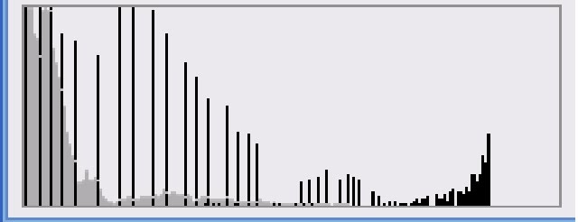
Figure 11: Histogram manipulated image and its corresponding grayscale PDF.The gray areas in the histogram corresponds to the PDF of the original image, whereas the darker areas correspond to the PDF of the new, manipulated image.

Enhancing an image is really fun especially if all the concepts and know hows have been understood. I'd like to thank my roommates, Arvin Mabilangan, Gino Leynes and Tino Borja for the support, encouragement and the intellectual debates. For technical correctness, I believe I got a score of 5. For quality of presentation, I will also give myself a grade of 5. But, since this is a late entry, I can't give myself the perfect score of 10/10, so all in all, I believe I deserve a grade of 9/10.